Lab 7: Rotating Apparatus 9/24

Purpose

In this lab we had to apply what we learned about circular motion to find the relationship between angular speed (ω) and the angle (θ) of the string for a rotating apparatus.

Procedure + Equipment

 

What we used: 

• tripod
• rotating motor
• string
• meter stick
• tall ring stand + clamp

What we did:

1. Measured the total height of the system, the length of the string, and the distance from the center of the system to the end where the string is tied. 
2. The professor then set the apparatus to rotate at 8 different speeds where we had to time for 10 rotations. We took times and h2 for each speed. 
3. The h2 was measured by setting up a ring stand with a paper, so that when the mass on the end of the string brushed against the paper, we could measure how the height of the paper to the ground

This is how we calculated h2, by adjusting the height of the paper until the mass at the end of the string brushed against the paper. Then that height was measured.

Data

On the left is the data we collected from the lab set up. On the right is the data was collected when timing for 10 rotations and the h2 for each trial. 

Calculations + Analysis

This is how we found the angle (θ) for each trial

This is how we calculated for f(θ) for each trial

This is how we calculated for the angular speed (ω) for each trial

This is what each θ , f(θ), and ω come out to be for each trial

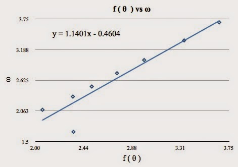
This is the slope we get when we graph f(θ) vs ω. Our slope is 1.1401.

The relationship we predicted we would get was 1, but we got 1.1401, which is 14.01% error.

Summary

In this lab we found the relationship between the angular speed (ω) and the angle (θ) of the string for the rotating apparatus. We  theorized that once we graphed it, the slope would be 1, but we found ours was 1.1401. That is a 14.01% error, and the reason for our percent error comes from the measurements we took for our data. We had some difficult times measuring the height and the distance of the set up. The time might also be off, which adds up.

Activity 2: Centripetal Acceleration 9/24

In this lab activity we measured an acceleration at different omegas (ω). The acceleration came from logger pro, and as a class we took the time for 3 rotations and took the average. We then graphed acceleration vs ω^2 and found the linear relationship, the slope, to be 0.1831+ 0.005.
The linear relationship is the radius of the circle. When measuring the radius we found that it was about 0.19 m. The calculated radius we found was 0.18 m + 5%.  The experiment proves the relationship between our acceleration and ω^2.

Our data along with the graph that shows the relationship between acceleration and ω^2. The equation a = Ax is similar to y = mx, where A is the slope. The slope is the radius of the circle.

Lab 6: Coefficients of Friction 9/17 - 9/22

Important Concepts

µs: The coefficient of static friction

fs: This is static friction - when the force of friction is greater than the applied force, also this force is needed to first move an object

fk: This is kinetic friction - the applied force is less to keep the object sliding as it breaks free from static friction. 

µk: The coefficient of kinetic friction

ex: It's harder to get a heavy object to move at first. but once it's sliding across the floor it seems easier as long as it keeps moving

Purpose

Part 1: In this part we found µs of a wooden blocks on a flat surface
Part 2:In this part of the lab, we used a force sensor to read the maximum and minimum static friction force of the blocks
Part 3: We had to find µs  of an object just before it starts to slide down an incline
Part 4: We found µk when an object is sliding down an incline
Part 5: We had to predict the acceleration and compare it with the measured acceleration of a two mass system 

 Procedure + Equipment

Part 1 - Static Friction (Cup + Water)
What we used:

• wooden blocks
• pulley
• styrofoam cup
• water + water dropper
• weights

What we did:

1. In this part of the lab, we weighed one block by itself, then two blocks together, until we weighed 4 blocks together
2. Then we took one wooden block and tied it to the pulley system 
3. On the other end of the pulley system we tied the styrofoam cup
4. We added water into the cup, and with the water dropper, we carefully added enough water until the block started to move
5. We weighed the mass of the cup and water
6. We repeated steps 3 and 4 until 4 blocks were at one end

Part 2 - Kinetic Friction (Force Sensor)
What we used:

• wooden blocks
• force sensor
• logger pro

What we did:

1. We first connected the force sensor to a weight and then calibrated by checking to see if logger pro was reading correctly
2. We then connected the force sensor to the wooden block with string and zeroed it when it was on the table. 
3. Then we pulled the block across the table at a constant speed, and collected the data
4. Step 4 was repeated with an extra block stacked on top until four blocks were on one side.

Part 3 - Coefficient of Static Friction (Angle)
What we used:

• ramp
• wooden block
• angle reader
• to measure the angle of the ramp

What we did:

1. We set up the ramp at a small incline and placed the wooden block at the top
2. The incline was increased until the wooden block started to slide
3. The angle of the ramp was recorded

Part 4 - Coefficient of Kinetic Friction (Angle)
What we used: 

• ramp
• wooden block
• angle reader
• we measure the angle of the ramp
• motion senor + logger pro 
• to measure the acceleration of the block 

What we did:

1. We set up the ramp at a new incline such that the block would accelerate
2. The motion sensor was placed at the top of the ramp
3. The lock was let go, and with logger pro we measured the acceleration

Part 5 - Predict Acceleration of a Two Mass System
What we used:

• ramp
• pulley 
• wooden block + hanging mass
• angle reader
• we measure the angle of the ramp
• motion senor + logger pro 
• to measure the acceleration of the block

What we did:

1. We set up the ramp at a new incline such that we could predict the acceleration by using the µk we found in part 4
2. The motion sensor went at the the bottom of the ramp
3. We measured the angle, and the mass of the wooden block and the hanging mass
4. The wooden block was tied to the pulley system and a hanging mass was on the other end 
5.  First we predicted the acceleration and then measured the acceleration with logger pro and compared those two. 

Data

Part 1

This is the data we collected that helped in finding what we had to graph

Part 2

This is the data we collected with the force sensor. The force sensor was able to give us the average kinetic friction force for the wooden blocks.

This is the data that we graphed to help us get kinetic friction

Part 3

 θ = 18º

Part 4

θ = 26º

Part 5 

m1 = 0.134 kg

m2 = 0.128 kg

θ = ? 

Calculations + Analysis

Part 1

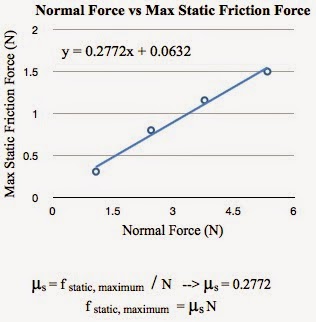
We graphed our data where the equation y = mx + b is similar to fs = µsN, where y = fs, m = µs, and x = N. This means that our slope m is our static friction for the block. We found the static friction of the block to be 0.2772.

Part 2

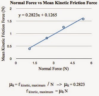
Similar to part 1, except with a constant acceleration applied to the block, we looked for the kinetic friction of the block. We found that the µs = 0.2823. 

Part 3

In this part of the lab, we had to solve for µs of the block on an inclined plane. We set up of the FBD and set up our equations and solved for µs, which was µs = tan(θ). We know the angle of the ramp and we found that the µs came out to be: 0.325
So, the coefficient of static friction for the block is 0.325. It's less than our µk because that is the force needed to get the block to slide.
Part 4

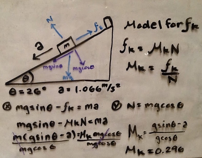
 In this part of the lab, the µk was solved for. We set up the FBD and set up our equations and solved for µk. The µk = gsin(θ) - a / gcos(θ), so our µk = 0.296
So, the coefficient for kinetic friction for the block is 0.296. It's less than our µs because it's already moving
Part 5 

We had to test out to see that if  with our calculated µk from part 4, we could calculate the acceleration of the block when it was on a two mass pulley system. Sadly, the angle for the incline wasn't measured, but we calculated what acceleration would be in terms of m1, m2, µk, and g.
We were also unable to measure the acceleration of the block, but seeing, so we have nothing to go off and compare to. 

Summary 

In this lab, we took a closer look at static and kinetic friction. This helped us better understand the two frictions and what their differences where. We were able to find and solve the coefficients of static and kinetic friction in two ways. Solving it by graphing our normal force vs our static/kinetic friction to get a slope that gave us the coefficients. We also solved for the coefficients using Newton's Law and the model of friction. 

In part 3 and part 4, we found the coefficient of static friction for the block is 0.325 and the coefficient for kinetic friction for the block is 0.296. We found that the µs was larger than the µk, and that is due to the force needed to move the object is greater than when the object is already in motion. 

Lab 5: Propagated Uncertainty 9/15

Purpose

In this lab we had to find the propagated uncertainties for the density of three cylinder metals and for a hanging mass.

Procedure + Equipment

Part 1 - Density

What we used:

• metal cylinders (brass, aluminum, and bronze)
• vernier caliper
• scale

This is a vernier caliper measuring the diameter of a metal cylinder

What we did: 

1. the diameter and height of each cylinder was measured in cm
2. the weight of the cylinders are measured in grams
3. density was calculated for each metal 

Part 2 - Hanging Mass
What we used:

• angle reader

What we did:

1. we took measurements of the lab set up for the hanging mass 
• we measured the tensions and the angles  

This is the set up for the hanging mass

Data

Part 1 - Density

This is the data we collected from measuring the metal cylinders

Part 2 - Hanging Mass

This is the data that was collected from the set up of the unknown hanging mass

Calculations + Analysis

Part 1 - Density

This is how we solved the equation of propagated uncertainty (dP) for density

This is the data table with the calculated numbers to get the propagated uncertainty in density

So, for the first part of the lab, we found the density and the propagated uncertainty for each metal cylinder. For copper: 9.08 g/cm^3 + 0.18 g/cm^3, for aluminum: 2.71 g/cm^3 + 0.06 g/cm^3, and for brass: 8.41 g/cm^3 + 0.13 g/cm^3.

Part 2 - Hanging Mass

This is how we found the equations for the unknown hanging mass and the propagated uncertainty (dm) for mass

This is the propagated uncertainty for the hanging mass

We found that the hanging mass was 0.75 kg and the propagated uncertainty was 0.032 kg.
So, the hanging mass is 0.75 kg + 0.032 kg.

Summary 

In this lab we learned how to find the propagated uncertainties by taking partial derivatives. We were able to find the propagated uncertainties of density for 3 metal cylinders and that of a hanging mass.
When we compare our calculated densities along with the propagated uncertainty, our answers come close to the actual densities of the metals. 

Lab 4: Projectile Motions 9/10

Purpose

In this lab, we determined the distance of a ball landing on a flat surface to help us predict where the ball would land on an inclined surface.

Procedure + Equipment

What we used:

•  v-channels
• the v-channel is a ramp shaped in a v, that allowed the ball to travel in a direct route 
• ring stand + clamp 
• the clamp holds the ring stand in place, so the v-channel can be inclined at an angle
• steel ball
• a steel ball is used to provide for a more accurate reading on the carbon paper
• carbon paper
• the carbon paper marked where the ball would land, allowing for the distance to be     measured 
• wooden ramp
• this is for the second part of the experiment where we have to predict where on the ramp the ball will land
• weights 
• to hold the wooden ramp in place

What we did:

1. we set up one v-channel at an incline connecting to another v-channel on a horizontal, this allowed the ball to travel in a direct route
2. carbon paper was placed in the general area where the ball landed
3. we placed the steel ball at the top again and let go
4. we measured the distance the ball traveled
5. we repeated steps 3 and 4 for a total of 5 trials
6. we measured the height from where the ball was launched
7. after this, through some calculations, we predicted where the ball would land if there was a ramp at the bottom 
8. part 2 was to do the experiment and see where the ball would land on the ramp.
9. we did the same as part 1 and did this for 5 trials

This is the set up for where the ball in launched from

Data

Part 1

This is the the distance the ball traveled when it landed on a flat surface

Part 2

This is the distance the ball traveled when it landed on a ramp. This data was collected after we calculated where the ball would land.

Calculations + Analysis

Part 1: This is how we calculated Vo, which came out to be 1.59 m/s

We were able to calculate a Vo to be 1.59 m/s from the data we collected. Given this Vo, we were then able to calculate where the ball would land when a ramp was placed at the bottom.

Part 2: This is how we calculated the distance (d) the ball traveled when it fell on the ramp.

We calculated that the ball would fall at 0.9072 m, but what we found was that on average the ball fell at 0.7636 m. Comparing these two value values, we find that the difference is a 19.42% error. This means that our experiment had some errors. There were some human errors in measuring the distance the ball fell. Another source of error could be from the set up, we had trouble with the v-channels shifting a bit during the experiments because they were not stable, and this could have affected the angle from where the ball was launched.

Summary

In this lab, we had to find an initial Vo for a ball in projectile motion and then calculate where the ball would land if there was a ramp at the bottom. We did the experiment and compared our theoretical value and our actual values and found our error was about 20%.

Lab 3: Falling Objects and Air Resistance 9/8

Purpose

In this lab, we will find the relationship between resistance force and speed using coffee filters and creating a model of f_air of a falling object.

Procedure + Equipment

What we used:

• coffee filters
• we dropped the coffee filters from a height and using logger pro, we were able to take a video and later analyze. 
• meter stick
• the meter stick was used to provide a reference for how fast the coffee filter was falling
• logger pro
• using logger pro, the videos were analyzed to give us the velocity of the falling coffee filters

What we did:

1. One person dropped one coffee filter from a height while someone else held the meter stick for reference. Another person was using logger pro and recorded a video as the coffee filter fell.
2.  Step one was repeated with an additional coffee filter until a total of five coffee filters were dropped.

 

Part 1: Data + Analysis

This is the video analysis on logger pro.

Video analysis for 1 filter

Video analysis for 2 filters

Video analysis for 3 filters

Video analysis for 4 filters

Video analysis for 5 filters

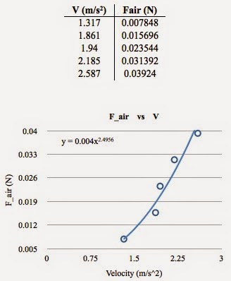
From the video analysis, we are given a time vs distance graph, but what is relevant are the slopes of the equation from each graph, which are the velocities of the coffee filters as they fall down. Knowing the mass of the coffee filters we then determined the air resistance force (f_air), which is mass x gravity.

This helped in finding what air resistance force is, which is mg.

These our values for air resistance force for each filter trial.

With the velocity and f_air known, we were then able to create a graph using a power fit. With the graph, we were then able to take the equation of the power law fit, which is y = 0.004x^2.4956. This equation is similar to what f_air is: kv^n.  

So, with our graph, we found the value for k = 0.004 and n = 2.4956.

This is the air resistance force vs velocity, which provides an equation of y = 0.004x^2.4956. The equation is similar to the equation F_resistance = kv^n, so our k is 0.004 and our n is 2.4956.

 Part 2: Data + Analysis

With our values of k and n we can create a model that shows the air resistance force of a falling object.

This data table is the modeling of f_air for a falling object.

Summary

In this lab we used coffee filters to record a video as they fell. We were then able to get a time vs distance graphs from the videos we analyzed, and from the slopes we were able to get each velocity. From that data and the calculated f_air, a velocity vs f_air graph was created to help us find the relationship. We found the equation: y = 0.004x^2.4956 which is our relationship.
So, we learned how to analysis a video on logger pro and found the relationship of a falling objects speed and air resistance force. We were also able to create a model of the falling objects from the values of k and n we found.

Activity 1: Non-Constant Acceleration

Purpose

In this lab we had to solve a non-constant acceleration problem both analytically and then numerically.

Problem Set-Up 

We want to know how far the elephant travels before stopping. We are solving for x.

Analytically

This is how we solved the problem using calculus. We found x = 248.7 m.

Numerically

We used excel to help solve the problem

This is the excel set up that helped in solving what x is

This is where the velocity changes, and that is where the answer lies. Somewhere between those two numbers. We found x = 248.628 m

Summary

We solved a problem both analytically and numerically. Our answers came out to be the same.

Questions

1.  Our answers were close to being the same
2. You know the time intervals are small enough when your computed answer is close to your calculated answer

Lab 2: Determining the Value of Gravity (g) 8/27

Purpose 

In this lab, we will determine the value of gravity (g) by using an apparatus consisting of an electro-magnet and spark generator.

Procedure + Equipment

On the left is the electromagnet. On the right is the apparatus that  provides the reading of the falling object. 

When the free fall object is held at the top by the electromagnet and then released, the spark generator then records the object’s position at every 1/60th of a second. This data is recorded on a strip of spark paper that shows each mark of the falling object. With the strip of paper, the distance of each mark can measured by aligning the 0cm mark of the meter stick with one of the dots. Each mark is then measured from the 0cm mark. This data gives us the time and the distance of the object as it fell. From the data collected, a data table was created with ∆X, the mid-interval time and speed. This allowed us to graph time vs distance and a velocity vs time. 

Data

Data collected from experiment and some calculations to help with graphing. 

This graph shows the relationship between distance and time. 

This is the velocity vs time graph. The slope of the equation of the graph gives us the acceleration  of the falling object. The acceleration is g, which is 963 cm/s².

Analysis + Calculations

With the velocity vs time graph we can find our value for g by finding the slope of the linear fit, which is an acceleration of 963 cm/s² , which is equivalent to 9.63 m/s². We know that the true value of g is 9.81 m/s², and the experimental value to be 9.63 m/s², so we can find the percent error. Using the formula % error = | true value - experimental value | / true value * 100% we find that the percent error is 1.83%. 

This data table shows each groups value of g when g is in m/s². From that data the average value of g was determined, along with the standard deviation. 

We also took each group's value of g and found that the class average for the value of g is 9.55 m/s². With this data we were also able to find the standard deviation.

Questions

1.  
2. The slope of the equation of the graph is the acceleration. This acceleration is your value for g. When comparing that value to the mean value, we find that our value of g falls within the 1st standard deviation. The mean value is 9.55m/s² + 0.1630. That means that the value for g should range from 9.387 m/s² and 9.713 m/s². Our value of g is 9.63 m/s², so it is within the desired range. 

   

   This shows where our value of g lies compared to the standard deviation.  It lies within the 1st standard deviation, so I believe it's still an acceptable value.

   When comparing our value to the actual value of g, we find a relative difference of -1.83%, and with the mean value we find a relative difference of -2.65%. This means that as a single group we had less of a difference when as a group.  
3. With the given equation, you have y=481.42x² + 138.04x - 0.0003. The derivative of the equation gives y'=962.84x + 138.04, so this equation gives you the acceleration. Compared to the other value of g, it is very close.

Summary

In this lab, we found the value of gravity (g) by using an electromagnet and spark generator. We used the position and time to get ∆x,  mid-interval time and speed. With that data we were able to graph a distance-time and velocity-time graphs. The graphs helped in deterring the value for g, which came to be 9.63 m/s². Then the values of each group's g was collected and used to determine the standard deviation. The standard deviation provided us with what values were closest to the mean value of g. We found that ours did lie close to the mean value with a percent error of 0.84%. This percent error tells us that our value was close to the experimental mean value for g. 

When taking the actual value of g to be  9.81 m/s², the relative difference is -1.83%. Our value of g was smaller than the actual value of g. There might be several reasons for the difference in our value of g compared to the actual value of g. Those reasons might be due to human error, somewhere along an error in measuring the distance of each mark could have been made. Another source of error is that in doing this, we aren't taking into account the air resistance.