Showing posts with label Labs. Show all posts

Wednesday, October 22, 2014

Lab 12: Collisions 10/15

Purpose

Procedure + Lab Equipment
Data

Calculations + Data Analysis
Conclusions

Thursday, October 16, 2014

Lab 11: Impulse-Momentum Theorem 10/13

Purpose
In this lab, we wanted to test if the impulse-momentum theorem is true - that impulse is equal to the momentum.
Procedure + Lab Equipment
What we used:
  • track
  • cart
  • clay + nail
    • the clay was placed on a wooden block and the nail on the force sensor - this was for the inelastic collision
  • logger pro 
    • force sensor + motion sensor
What we did:
Part 1 - Elastic Collision (bouncing)
  1. on one end of the track, a spring was placed at the end 
  2. at the other was the motion sensor
  3. the force sensor was attached to one end of the cart
  4. the cart with the force sensor is then weighed
  5. the force sensor was calibrated and then placed on the cart
  6. data was collected as the cart is pushed into the spring
  7. this is repeated with an additional mass on the cart
Part 2 - Inelastic Collions
  1.  the same as part one, except the spring is changed with clay
  2. a nail is attached to the end of the force sensor
Data
Part 1 -Elastic Collision
This is the data for the cart
This is the data for the cart with an additional mass
 Part 2 - Inelastic Collision
This is the data for when the cart collides with the clay
Calculations + Data Analysis
Using the equations of momentum, we were able to calculate the momentum of the cart and compare it to the impulse of the cart.
Conclusion
We found that the theorem is true....

Tuesday, October 14, 2014

Lab 10: Magnetic Potential Energy 10/8 - 10/13

Purpose
In this lab, we are using the relationship between force and distance to find the potential energy of the magnet and see that the conservation of energy applies to this system as well.


Procedure + Lab Equipment
What we used:
  • air track + vacuum
  • glider cart
  • angle reader 
  • motion sensor
What we did:
  1. We placed the air track at an angle (day 1)
    • we let the glider go measured how far away the glider was from the  magnet
    • we repeated this step at different angles for a total of 5x
  2. We  leveled the track and then gave the glider a push toward the magnet (day 2)
Data
The graph is the relationship between the force and the distance
This graph shows how as the angle of the ramp is increased, the force increases as well, and the distance between the magnets decreases. This force and distance relationship helps us in finding the potential energy as a function of distance. So as the distance between the magnet changes, so does the potential energy. 
This is the data for the cart when the track is leveled
This is the data collected for the cart as it approached and moves away from the magnet.
Calculations + Data Analysis
This is the data for energy at each point
This is the graph that shows the PE and KE as the glider approaches and then moves away from the magnet.


Summary


Monday, October 6, 2014

Lab 9: Conservation of Energy in a Mass-Spring System 10/6

Purpose
In this lab, we measured the kinetic energy (KE)  and gravitational potential energy (GPE) for the mass and spring, and elastic potential energy (EPE) for the spring to verify that energy is conserved through out the system.
Procedure + Lab Equipment
What we used:
  • ring stand + clamp
  • spring
  • mass
  • ruler
  • logger pro 
    • motion sensor + force sensor
This is the lab set up for when the spring is stretched, below is the motion senor
What we did: 
  1.  we used the motion sensor to record the height of the spring when it was not stretched and when it was stretched
  2. we attached the top end of the spring to the force sensor and hung the mass at the other end of the spring
  3. we weighed the spring 
  4. we then took the final reading as the mass was hung on the spring
Data
With logger pro, we were able to record the velocity of the spring as it moved
This is the height without and with the mass, and the mass of the spring is 0.044kg
The slope is the k constant of the spring
show integration work 
Calculations + Data Analysis
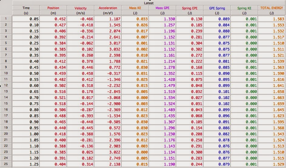
The data table that calculates KE, GPE, EPE, and Total Energy at each point as the spring oscillated from stretched to not stretched
This is the data table we created to find KE,  GPE, and EPE of the mass and spring at each point as the spring oscillated between stretched and not stretched. We then took those numbers and created a column for the total energy at each point. From the data table we see that the total energy through out the system appears to be consistent. 
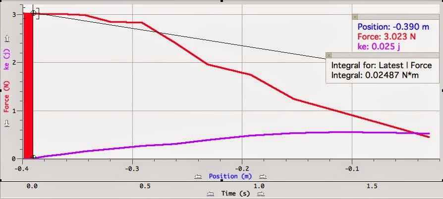
From this graph we can see that when the spring is stretched, the total energy stays consistent, unlike when it bounces back up.
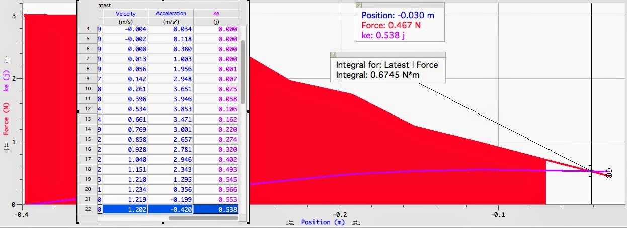
From this graph, we can actually see a clearer picture-that energy is consistent at every point as the spring goes from not stretched to stretched.
Summary
In this lab, we wanted to verify that in a mass-spring system, that the conservation of energy was true. We used logger pro to measure the velocity and position over a period of 10 seconds to help us find the energies at each point. Our graph showed that the energy was consistent throughout those 10 seconds, so, we were able to verify the conservation of energy in a mass-spring system.

Friday, October 3, 2014

Lab 8: Work-KE Theorem 10/1 - 10/6

Purpose
In this lab, we wanted test our hypothesis that, based on the work-kinetic energy theorem, the work done on the spring is equal to the kinetic energy of the spring.
Procedure + Lab Equipment
What we used:
  • cart + block
  • ramp
  • spring
  • logger pro
    • force sensor + motion sensor 
This is the lab set up for the experiment when the spring is at rest
What we did:
  1. the mass of the cart + block was measured
    • attached one end of the spring to the cart
  2. calibrated the force sensor
    • we then connected the force sensor to the other end of the spring and let the spring at rest and zeroed
  3. stretched the spring and let go - recorded the data
Data
Graph 1
Graph 2
Graph 3
Graph 4
Calculations + Data Analysis
Kinetic energy is found through... 
This is how the kinetic energy is found.
These are the percent errors for their respective graphs
We can see that throughout the graph, work is close to equal to the kinetic energy. So, we found that the work-kinetic theorem to be true.  
Summary
In this lab, we set out to test if the work-kinetic energy theorem is true. We used a cart-spring system to see if the work done was equal to the kinetic energy. Our data shows that work was close to equal to the kinetic energy. We aren't going to get exact numbers due to some errors. Our spring was resting on something, as can be seen in the lab set up. This may have affected our data. 
Though are numbers weren't exact, they did let us see that the work-kinetic energy theorem works. 

Monday, September 29, 2014

Lab 7: Rotating Apparatus 9/24

Purpose
In this lab we had to apply what we learned about circular motion to find the relationship between angular speed (ω) and the angle (θ) of the string for a rotating apparatus.
Procedure + Equipment
 
What we used: 
  • tripod
  • rotating motor
  • string
  • meter stick
  • tall ring stand + clamp
What we did:
  1. Measured the total height of the system, the length of the string, and the distance from the center of the system to the end where the string is tied. 
  2. The professor then set the apparatus to rotate at 8 different speeds where we had to time for 10 rotations. We took times and h2 for each speed. 
  3. The h2 was measured by setting up a ring stand with a paper, so that when the mass on the end of the string brushed against the paper, we could measure how the height of the paper to the ground
This is how we calculated h2, by adjusting the height of the paper until the mass at the end of the string brushed against the paper. Then that height was measured.
Data
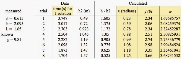
On the left is the data we collected from the lab set up. On the right is the data was collected when timing for 10 rotations and the h2 for each trial. 
Calculations + Analysis
This is how we found the angle (θ) for each trial

This is how we calculated for f(θ) for each trial
This is how we calculated for the angular speed (ω) for each trial
This is what each θ , f(θ), and ω come out to be for each trial
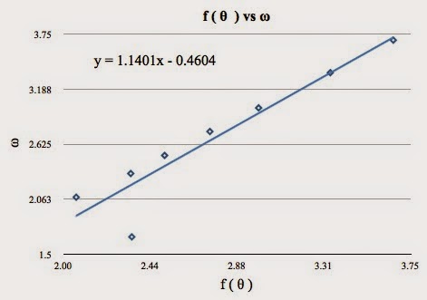
This is the slope we get when we graph f(θ) vs ω. Our slope is 1.1401.
The relationship we predicted we would get was 1, but we got 1.1401, which is 14.01% error.

Summary
In this lab we found the relationship between the angular speed (ω) and the angle (θ) of the string for the rotating apparatus. We  theorized that once we graphed it, the slope would be 1, but we found ours was 1.1401. That is a 14.01% error, and the reason for our percent error comes from the measurements we took for our data. We had some difficult times measuring the height and the distance of the set up. The time might also be off, which adds up.

Saturday, September 20, 2014

Lab 6: Coefficients of Friction 9/17 - 9/22

Important Concepts
µs: The coefficient of static friction
fs: This is static friction - when the force of friction is greater than the applied force, also this force is needed to first move an object
fk: This is kinetic friction - the applied force is less to keep the object sliding as it breaks free from static friction. 
µk: The coefficient of kinetic friction
ex: It's harder to get a heavy object to move at first. but once it's sliding across the floor it seems easier as long as it keeps moving
Purpose
Part 1: In this part we found µs of a wooden blocks on a flat surface
Part 2:In this part of the lab, we used a force sensor to read the maximum and minimum static friction force of the blocks
Part 3: We had to find µs  of an object just before it starts to slide down an incline
Part 4: We found µk when an object is sliding down an incline
Part 5: We had to predict the acceleration and compare it with the measured acceleration of a two mass system 
 Procedure + Equipment
Part 1 - Static Friction (Cup + Water)
What we used:
  • wooden blocks
  • pulley
  • styrofoam cup
  • water + water dropper
  • weights
What we did:
  1. In this part of the lab, we weighed one block by itself, then two blocks together, until we weighed 4 blocks together
  2. Then we took one wooden block and tied it to the pulley system 
  3. On the other end of the pulley system we tied the styrofoam cup
  4. We added water into the cup, and with the water dropper, we carefully added enough water until the block started to move
  5. We weighed the mass of the cup and water
  6. We repeated steps 3 and 4 until 4 blocks were at one end
Part 2 - Kinetic Friction (Force Sensor)
What we used:
  • wooden blocks
  • force sensor
  • logger pro
What we did:
  1. We first connected the force sensor to a weight and then calibrated by checking to see if logger pro was reading correctly
  2. We then connected the force sensor to the wooden block with string and zeroed it when it was on the table. 
  3. Then we pulled the block across the table at a constant speed, and collected the data
  4. Step 4 was repeated with an extra block stacked on top until four blocks were on one side.
Part 3 - Coefficient of Static Friction (Angle)
What we used:
  • ramp
  • wooden block
  • angle reader
    • to measure the angle of the ramp
What we did:
  1. We set up the ramp at a small incline and placed the wooden block at the top
  2. The incline was increased until the wooden block started to slide
  3. The angle of the ramp was recorded
Part 4 - Coefficient of Kinetic Friction (Angle)
What we used: 
  • ramp
  • wooden block
  • angle reader
    • we measure the angle of the ramp
  • motion senor + logger pro 
    • to measure the acceleration of the block 
What we did:
  1. We set up the ramp at a new incline such that the block would accelerate
  2. The motion sensor was placed at the top of the ramp
  3. The lock was let go, and with logger pro we measured the acceleration
Part 5 - Predict Acceleration of a Two Mass System
What we used:
  • ramp
  • pulley 
  • wooden block + hanging mass
  • angle reader
    • we measure the angle of the ramp
  • motion senor + logger pro 
    • to measure the acceleration of the block
What we did:
  1. We set up the ramp at a new incline such that we could predict the acceleration by using the µk we found in part 4
  2. The motion sensor went at the the bottom of the ramp
  3. We measured the angle, and the mass of the wooden block and the hanging mass
  4. The wooden block was tied to the pulley system and a hanging mass was on the other end 
  5.  First we predicted the acceleration and then measured the acceleration with logger pro and compared those two. 
Data
Part 1
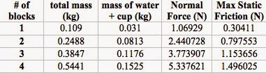
This is the data we collected that helped in finding what we had to graph
Part 2
This is the data we collected with the force sensor. The force sensor was able to give us the average kinetic friction force for the wooden blocks.
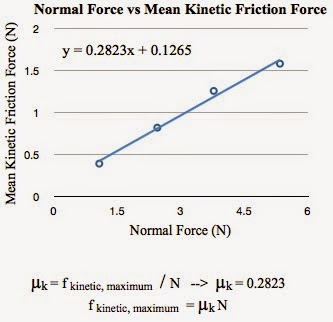
This is the data that we graphed to help us get kinetic friction
Part 3
 θ = 18º
Part 4
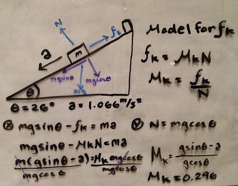
θ = 26º
Part 5 
m1 = 0.134 kg
m2 = 0.128 kg
θ = ? 
Calculations + Analysis
Part 1
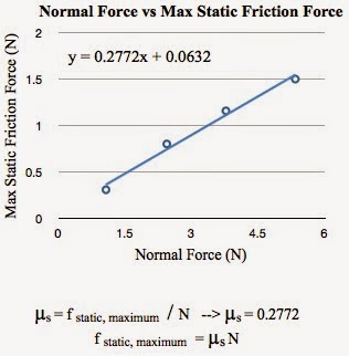
We graphed our data where the equation y = mx + b is similar to fs = µsN, where y = fs, m = µs, and x = N. This means that our slope m is our static friction for the block. We found the static friction of the block to be 0.2772.
Part 2
Similar to part 1, except with a constant acceleration applied to the block, we looked for the kinetic friction of the block. We found that the µs = 0.2823. 
Part 3
In this part of the lab, we had to solve for µs of the block on an inclined plane. We set up of the FBD and set up our equations and solved for µs, which was µs = tan(θ). We know the angle of the ramp and we found that the µs came out to be: 0.325
So, the coefficient of static friction for the block is 0.325. It's less than our µk because that is the force needed to get the block to slide.
Part 4
 In this part of the lab, the µk was solved for. We set up the FBD and set up our equations and solved for µk. The µk = gsin(θ) - a / gcos(θ), so our µk = 0.296
So, the coefficient for kinetic friction for the block is 0.296. It's less than our µs because it's already moving
Part 5 
We had to test out to see that if  with our calculated µk from part 4, we could calculate the acceleration of the block when it was on a two mass pulley system. Sadly, the angle for the incline wasn't measured, but we calculated what acceleration would be in terms of m1, m2, µk, and g.
We were also unable to measure the acceleration of the block, but seeing, so we have nothing to go off and compare to. 
Summary 
In this lab, we took a closer look at static and kinetic friction. This helped us better understand the two frictions and what their differences where. We were able to find and solve the coefficients of static and kinetic friction in two ways. Solving it by graphing our normal force vs our static/kinetic friction to get a slope that gave us the coefficients. We also solved for the coefficients using Newton's Law and the model of friction. 
In part 3 and part 4, we found the coefficient of static friction for the block is 0.325 and the coefficient for kinetic friction for the block is 0.296. We found that the µs was larger than the µk, and that is due to the force needed to move the object is greater than when the object is already in motion. 

Wednesday, September 17, 2014

Lab 5: Propagated Uncertainty 9/15

Purpose
In this lab we had to find the propagated uncertainties for the density of three cylinder metals and for a hanging mass.
Procedure + Equipment
Part 1 - Density
What we used:
  • metal cylinders (brass, aluminum, and bronze)
  • vernier caliper
  • scale
This is a vernier caliper measuring the diameter of a metal cylinder
What we did: 
  1. the diameter and height of each cylinder was measured in cm
  2. the weight of the cylinders are measured in grams
  3. density was calculated for each metal 
Part 2 - Hanging Mass
What we used:
  • angle reader
What we did:
  1. we took measurements of the lab set up for the hanging mass 
    • we measured the tensions and the angles  
This is the set up for the hanging mass
Data
Part 1 - Density
This is the data we collected from measuring the metal cylinders
Part 2 - Hanging Mass
This is the data that was collected from the set up of the unknown hanging mass
Calculations + Analysis
Part 1 - Density
This is how we solved the equation of propagated uncertainty (dP) for density

This is the data table with the calculated numbers to get the propagated uncertainty in density

So, for the first part of the lab, we found the density and the propagated uncertainty for each metal cylinder. For copper: 9.08 g/cm^3 + 0.18 g/cm^3, for aluminum: 2.71 g/cm^3 + 0.06 g/cm^3, and for brass: 8.41 g/cm^3 + 0.13 g/cm^3.

Part 2 - Hanging Mass
This is how we found the equations for the unknown hanging mass and the propagated uncertainty (dm) for mass
This is the propagated uncertainty for the hanging mass
We found that the hanging mass was 0.75 kg and the propagated uncertainty was 0.032 kg.
So, the hanging mass is 0.75 kg + 0.032 kg.
Summary 
In this lab we learned how to find the propagated uncertainties by taking partial derivatives. We were able to find the propagated uncertainties of density for 3 metal cylinders and that of a hanging mass.
When we compare our calculated densities along with the propagated uncertainty, our answers come close to the actual densities of the metals.